Create Your Own Neural Network From The Scratch (A.I - 101)

[Kuchwizzy]

Watu wengi naona hawana interest na concept za kuumiza kichwa, ila kwasababu Artificial intelligence ndio future, huu uzi utakuwa guide kwa yoyote atakayekua interested in the future

 

[Kuchwizzy]

Kama una pay attention, kila lecture ina add level yake of complexity
Lakini sio kwasababu concepts zenyewe ni ngumu, ila ni kwamba kuna concepts nyingi sana ndogo ndogo ambazo tunapaswa kuzielewa zina fit vipi kwenye overall picture

 

[Kuchwizzy]

Kama sipo peke yangu humu ndani, nakaribisha maswali, comment au chochote tuu keep uzi active

 

[Kuchwizzy]

Amini usiamini, mwisho wa lecture tutakua na working non trivial neural network model ambayo tunaielewa nje ndani

 

[Kuchwizzy]

Mda huu unaweza kupitia notes zako za Calculus za mwarami, tutaitumia mbeleni

 

[Kuchwizzy]

Mbona MMU kupo active sana?

 

[Andazi]

Part 09 - Learning Weights From More Than One Node​

Upo lecture ya ngapi?

Ya 4 ila narudia rudia sana maana dah

 

[Andazi]

Mda huu unaweza kupitia notes zako za Calculus za mwarami, tutaitumia mbeleni

Nilipita kimzaba mzaba sielewi kitu kwenye hii topic

 

[Andazi]

Mbona MMU kupo active sana?

Mkuu kule kuna watu wapenda ngono alafu humu ni watu wanaojitesa ili warahisishe maisha ya wengine

 

[Hamritzer]

Watu wengi naona hawana interest na concept za kuumiza kichwa, ila kwasababu Artificial intelligence ndio future, huu uzi utakuwa guide kwa yoyote atakayekua interested in the future

Safi sana mkuu, tupo pamoja

 

[adriz]

Mbona MMU kupo active sana?

Tatizo wengine tuliscore "F" za mathe kwa hiyo hapa tunaona chenga tu.

 

[Kuchwizzy]

Part 10 - Backpropagating Errors with Matrix Multiplication​

Kabla sijaendelea, nimeona ni muhimu ku summarize operations kuu mbili zinazofanywa na kila node kwenye neural network

Kila node, unaweza kuitazama kama independent computing unit inayofanya operations kubwa kwenye input inayopokea

1. Operation ya kwanza
Ni linear transformation through multiplication of weights and input matrices, output ya hii operation ni matrix ya combined and moderated input kama tulivyoona kwenye lectures zilizopita

2. Operation ya pili
Ni non linear transformation kwa ku apply activation function kwenye kila element ya combined and moderated input matrix, kupata output matrix yake (ya hio node)

Hii process inafanywa na kila node ya hidden layer na output layer
Hii hatua ya kwanza inajulikana kama Forward pass


Baada ya ku calculate error, hatua inayofata ni kusafirisha (propagate) errors zilizopatikana back to the network, from kila node ya hidden layer mpaka nodes zote za input layer
Hii hatua ya pili inajulikana kama backpropagation


Nimechora hivi vielelezo kukazia hii point

Sasa, kwenye lecture iliyopita, tumeona ni jinsi gani tunaweza tumia mbinu nyingine ya ku compute error ya hidden layer licha wa kutojua obvious target value inayopaswa kuwa predicated na hio node

Formula ilikua ni hii, tuchukulie mfano wa hidden node inayosafirisha signals kwenda kwenye output nodes mbili
kama inavyoonyeshwa na hiki kielelezo

Split errors zinazokua propagated to hii node zinapatikana kama jumla ya:

na:

Now, tuki add hizo spilt errors zinazokua propagated back to node yetu, tunapata:

So, error ya node yoyote ile kwenye hidden layer during backpropagation inapatikana kwa hio formula
Zitakazo ongezeka tu ni number of weights na errors depending on number of output node connected back
lakini main operation inabaki vile vile bila kujali tuna output nodes 2 au zaidi

Same concept ina apply kwenye hidden node ya pili, split errors ni

na

Tuki add

Lakini tushajifunza kuwa, kwa ku write hizi parameters kama matrix, kuna advantage kubwa mbili tunazipata

Kukukumbusha tu, advantage ya kwanza ni kuwa, inakua rahisi kuandika mathematical expressions tunazotumia kwenye calculations, mbili tunatake advantage ya hardware za computers ambazo zipo haraka zaidi kwenye matrix multiplication kwa sababu ya nature tu ya matirx.

So hebu tujaribu kuandika hio expression kama matrices
Tuanze na output errors, E1 na E2, hizi tunaweza kuziweka ni matrix kama ifatavyo

Tujaribu pia kuziweka errors zote za hidden layer nzima kwenye mtindo wa matrix

But what if tuki arrange kwa kutumia full expressions tulizotoka ku discuss hapo mwanzo

NOTE : Kwenye kupanga hizi parameters kama matrix, hakuna formula yoyote inayotumika, ni order ya mpangilio tunayoamua kuitumia ndio ina matter

Mfano hapo juu, tumeamua kuweka weights associated with split errors za node ya kwanza kwenye row ya kwanza
Na zile weights associated with split errors za node ya pili kwenye row ya pili

Kwenye matrix ya pili, tumeweka errors kutoka kwenye output nodes, ni just ordering.

Sasa tumepata matrix expression tulizokua tunazihitaji, lakini tunataka iwe simple zaidi ya hapo ili hizo denominators zisitusumbue wakati wakupiga mahesabu
Ni kweli ukitazama utaona jinsi gani hizo denominators zimefanya matrix epression isiwe rahisi kuliko tunavyotaka iwe

Hapa kuna genius assumption tunayoweza kuitumia, ngoja tuione hii assumption in action halafu tutaielezea
Tunaweza tukaondoa kabisa hizo denominators zote kwenye matrix ya kwanza ili kupata hii expression rahisi zaidi

Unaweza kujiuliza tumefanya "maajabu" gani hapa?
Kwanza nikutoe hofu hakuna kanuni yoyote ya hesabu iliyokiukwa hapa, tunachofanya hapa ni ku arrange tu parameters zetu ziwe kwenye matrix expression rahisi ambayo sisi tunaweza kufanya nayo kazi

Cha msingi ni kujua maana ya kila parameter yetu na consequence ya maamuzi tunayoyachukua
Sasa tutazame logical assumption tuliyotumia hapa:


Kama unakumbuka kwenye lecture iliyopita, lengo lilikua ni ku split error kulingana na magnitude of weight ambayo hio node imechangia kwenye overall error, kazi ya zile denominators ilikua ni ku normalize au kusawazisha error tunayo attribute kwenye node kulingana na contribution of error iliyofanywa na node nyingine

Lengo lilikua ni kuhakikisha kila hidden node inapata its "FAIR" share of error kulingana na mchango wake kwenye overall error, so hizo denominator kwa maana nyingine zilikua ni just normalizing factor

So kama tuki remove normalizing factor, tutakua tuna propagate more or less error kwenda kwenye hidden node kuliko inavyotakiwa lakini but still tutakua tuna propagate error back to the node in proportional to its weight kitu ambacho ndio cha muhimu zaidi.

Huu ni mfano, suppose weights zetu ni 0.6 na 0.2, zote zime contribute error ya 2.0
with normalizing factor, split error kwenda kwenye node yenye weight ya 0.6 itakua

Na split error kwenda kwenye node yenye weight 0.2 itakua:

so tuna propagate more error kwenda kwenye node iliyo contribute more weight (iliyokua na influence zaidi kwenye output ya output node)

Bila normalizing factor, split error kwenda kwenye node yenye weight ya 0.6 itakua

Na split error kwenda kwenye node yenye weight 0.2 itakua:

Kama unaona, hata bila normalizing factor, still tuta propagate more error kwenye node iliyo cotribute more weight
Tofauti ni kwamba bila normalizing factor, tuna loss some accuracy / tunapoteza usahihi fulani kwenye errors tunazo propagate
Logic ya hii assumption ni kwamba, hata kama tuta propagate slightly inaccurate errors, neural network yenyewe over time ita correct makosa yetu tuliyo introduce kwa ku remove normalizing factor
So we are still good.
Unakumbuka hii matrix tuliyokuja nayo kwenye Lecture 7 ? tuliona ni weights matrix kati ya hidden layer na output layer

Linganisha na hii

NOTE : Unaweza kutumia square brackets au parentheses ku donote matrices, ni kitu kile kile

Ukitazama kwa makini utagundua matrix ya pili (kwenye error_hidden) ni transposing of matrix W
Tume switch row kuwa column tu

The transpose of a matrix is simply a flipped version of the original matrix. We can transpose a matrix by switching its rows with its columns. We denote the transpose of matrix AA by AT

Generally, transpose of any matrix, X

is given by

So tunaweza ku rewrite expression yetu kama

So, generally, error ya hidden layer ya neural network yenye ukubwa wowote ule ni product ya transpose of matrix ya weights kati yake na layer inayofata na errors matrices za layer hio inayofatia

Tuchukue mda huu, ku summarize yote tuliyojifunza so far.

Key Points Summary:

• Backpropagation as Matrix Multiplication: Backpropagation, the process of calculating error gradients in neural networks, can be efficiently represented and computed using matrix operations.
• Conciseness and Efficiency: Matrix representation provides a compact way to express backpropagation regardless of the network's size. It also enables programming languages with matrix computation capabilities to perform these calculations faster and more efficiently.
• Overall Efficiency: Both the forward pass (feeding signals through the network) and the backward pass (backpropagation of errors) can be optimized using matrix calculations, leading to improved computational efficiency in neural network training.

Definition: Transpose of a Matrix and normalizing factor

• The transpose of a matrix is obtained by interchanging its rows and columns. In other words, if the original matrix is of size m x n (m rows and n columns), its transpose will be of size n x m.
• A normalizing factor is a value used to scale or adjust a set of numbers so that they fall within a desired range or have a specific total sum

Next: How Do We Actually Update Weights?

 

[Kuchwizzy]

Part 11 - How Do We Actually Update Weights?​

Tumefika kwenye hatua muhimu sana ya hii series, How do we actually update weights?

Kumbuka, kama ilivyokua slope kwenye linear classifier, kwenye neural network, ni weight ndio inayo learn
Hivyo basi, kama tukiweza ku update weight, itupe target value tunayohitaji, tutakua tumefanikiwa ku train neural network

Lakini kuna tatizo, kwenye linear classifier, output yake ilikua inategemea kwenye parameter moja tu, slope
So, ku change output au prediction ili iwe sawa au ikaribie target value, tulichokua tunafanya ni just ku adjust kidogo kidogo value ya single variable / parameter ambayo ilikua slope yetu

Na tukaweza ku come up na hii expression kwenye Lecture 3

Tatizo lenyewe ni kwamba, kwenye neural network, output ya network nzima ina depend kwenye parameters zaidi ya moja. ambazo ni weights
So kitendo cha ku adjust hata weight moja, hata kwa kiasi kidogo, kunaweza change output yetu katika namna ambayo hatuwezi ku predict

Chukulia mfano wa simple deep neural networks, yenye layers tatu, kila layer ikiwa na node tatu

Utaona kuwa, output ina depends kwenye variables 18

Na hio ni very simple deep neural network, for very intelligent models tunaweza kuwa na mamia au maelfu ya hidden layers, kila layer ikiwa na mamia au maelfu ya nodes

Mbaya zaidi ni kwamba, kuna operations tunazifanya katikati (Linear & non linear transformation)
Hii inafanya output yetu iwe function ya function ya function ya function and so....

Tuelezee hio point hapo juu mathematically tuone ilivyo ngumu,

Output matrix ya network yoyote ile (yenye any number of layers and nodes) tunaipata kwa hii expression
(Tunajua hassle tulizopitia mpaka kupata hii expression rahisi)

Huku

ikiwa ni output matrix ya last hidden layer

Lakini kumbuka tunafanya Layer-wise computation, where each layer's result becomes the input for the following layer
So

ni function ya output matrix kutoka kwenye previous hidden layer (kwa 3 layers Neural Net (NN) ni input layer), so

Kama tungekua na more than one hidden layer, tungeendelea kufanya hivi hivi up to input layer

Kwa simple 3 layers neural network, output matrix O, ni

Kumbuka pia

Huku I ikiwa ni Input matrix kwenye hio layer ambayo nayo ni output kutoka kwenye layer nyingine so ni function pia ya function nyingine kama tuna more than one hidden layer
Kumbuka pia sigmoid ni:

So kuna so many combinations of weights ambazo hatuwezi hata ku imagine
For very simple 3 layers NN, hii ndio full version ya function yake:

So hatuwezi kutumia hesabu yoyote ku directly solve aina hii ya function

Hebu, tu attempt brute force method, kama hackers tuna try ku crack hii password

Swali la msingi tunalopaswa kujiuliza, je tunaweza ku try every possible combinations of all weights kwenye network yetu mpaka tutakapopata combination of weights ambayo itatuleta karibu na target value?

Fikiria tu kuwa, weight moja inaweza kuwa na 1,000 possible values kati ya 1 na -1, kama 0.567, 0.345 etc
Na kwa neural network yetu hapo juu, tuna 18 weights, so tunazungumza kuhusu 18,000 combinations kwa neural network rahisi kama hio

Kama tuna NN yenye 500 nodes (hii ni neural network ya kawaida sana) tutakua na 500 millions possible weight combination za kujaribu, hii tutatumaia miaka 16 kujaribu hizo possible zote, na hio ni for just one training example

Vipi kama tuna 1,000 examples, tutazungumza kuhusu miaka 16,000


So hatuwezi kutumia Algebra directly ku solve hili tatizo, na wala hatuwezi kutumua Brute force algorithm
Hili lilikua fumbo kubwa kwa mathematicians, na iliwachukua miaka mingi mpaka walipopata ufumbuzi

Ladies and gentlemen, let me introduce you to Gradient Descent Algorithm , jawabu la fumbo letu hapo juu
Ni mchawi mmoja wa namba kwa jina la Augustin-Louis Cauchy
Ndio aliyekuja na hio mbinu.

Hii Algorithm, kama tunavyokwenda kuiona, ni moyo wa successfully Machine Learning Models zote duniani
From GPT, to Gemini, to LLMA to SORA.

Na hii ndio final step, itakayotupa final equation, ambayo tuta combine na equations zilizopita ku build sasa neural network model

ANGALIZO tu, kwasasa tunapandisha mlima wa hesabu, so pay attention na funga mkanda wa siti yako.

Hizi concepts zote tulizo zitumia mpaka sasa, ni zao la watu wenye akili possibly kuliko sisi (from mathematicians, computer scientists, wanafizikia na engineers), ambao wali spend mda mrefu kuziweka pamoja

Tutumie mda huu ku summarize vya msingi tulivyojifunza

Gemini 1.5 pro, ime summarize uzuri yote tuliyojifunza kwenye hii essay:

What is a Brute Force Algorithm?

A brute force algorithm is a straightforward problem-solving approach that systematically tries every possible solution until it finds the correct one or the best one according to some criteria. It doesn't rely on any clever optimizations or shortcuts but instead exhausts the entire search space.

How to Train a Neural Network by Trying Every Possible Combination of Weights (in Theory)

In the context of neural networks, a brute-force approach would involve:

1. Defining the search space:
   • Set a range for each weight in the network (e.g., between -1 and 1).
   • Discretize this range into a finite number of possible values (e.g., increments of 0.01).
   • This creates a finite, albeit potentially massive, set of all possible weight and bias combinations (tutakuja kuona nini maana ya bias hapo mbele, ila for now, ni just parameter kama ilivyo weight).
2. Iterating through combinations:
   • Systematically try each combination of weights.
   • For each combination, evaluate the network's performance on the training data using a loss function (error function)
   • Keep track of the combination that yields the lowest loss / error.
3. Selecting the best combination:
   • Once all combinations have been tried, the one with the lowest loss is considered the "best" and is used as the final set of weights for the neural network.

Why You Shouldn't Train a Neural Network this Way (in Practice)

• Computational Infeasibility: Even for small neural networks, the number of possible weight combinations is astronomical. Trying them all would take an impractical amount of time, even with powerful computers.
• Inefficiency :Brute force is highly inefficient. There are far more sophisticated optimization algorithms (like gradient descent and its variants) that intelligently navigate the search space, finding good solutions much faster.
  
  
• Overfitting: Brute force is prone to overfitting. It might find a combination that performs perfectly on the training data but fails to generalize to new, unseen data.

Conclusion
While it's theoretically possible to train a neural network using a brute force approach, it's practically infeasible and inefficient. Modern optimization techniques are vastly superior in terms of both speed and the quality of the solutions they find.

Next : Gradient Descent Algorithm

 

[Kuchwizzy]

Uzi umekimbiwa huu, naweza post video ya utupu humu na watu wasijue.

 

[Kuchwizzy]

Kwa mtakao ufatilia huu uzi in the future, kila lecture ina link yake kwenye post ya kwanza
Na overtime tutakua tuna update hizo lectures kama kuna pahala hakupo sawa, au maelezo hayajitoshelezi

 

[Artificial Horizon]

Research yangu ya Undergraduate kuhusu "The influence of river sinousity on self purification capacity of river streams"
Nilitaka kutengeneza modal kwa kutumia neural links kwa vile nilikuwa najua python kidogo😂
Ndugu zangu mbona niliona nyota acha nile shule hapa niongeze maarifa.

 

[Kuchwizzy]

Research yangu ya Undergraduate kuhusu "The influence of river sinousity on self purification capacity of river streams"
Nilitaka kutengeneza modal kwa kutumia neural links kwa vile nilikuwa najua python kidogo😂
Ndugu zangu mbona niliona nyota acha nile shule hapa niongeze maarifa.

I really encourage you to read lectures zote...at your pace

 

[Nicklaus]

Nili practice baadhi neural networks, kama CNN, ila sikuwa naelewa kitu gan kipo nyuma yake. Kupitia huu uzi umenifungua mambo mengi.
Endelea kutoa elimu tuelimike.

 

[Kuchwizzy]

Part 12 - Gradient Descent Algorithm​

Kwenye Lecture iliyopita tuliona ni jinsi gani ilivyo ngumu kurekebisha (adjust) kila weight kwenye neural network nzima based on feedback errors zinazokuwa propagated back to the network wakati wa backpropagation

Kwa simple linear classifier, yenye parameter moja, ilikua rahisi kutafuta mahusiano kati ya Error

na kwa kiasi gani inapaswa kurebisha thamani ya parameter

ku reduce error, tofauti kati ya network predicated value (output) na target value, kupitia hii formula

Kwasababu output ya network nzima, ina depend on only one parameter, ambayo tunaweza kui tweak kwa urahisi

Tatizo kuhusu neural network, ni kwamba output ina depend on many parameters, weights huku kila weight ikiwa na influence kwenye output ambayo imekua influenced pia na weight nyingine
Hii inafanya final output ya neural network iwe ni function of functions (multivariate function), hivyo huwezi kuifanya weight

iwe subject of this function kwa kutumia linear algebra.

Na hatuwezi ku try every possible values of weights kupata correct values of weight through brute force kama tulivyoona.

Solution ya hili tatizo ni Gradient Descent Algorithm ambayo tunaenda kuitazama kwenye hii lecture.

Kabla hatujaendelea, tukumbuke kuwa, Error

ni tofauti kati ya network output

na target value

So, kama output ya neural network ni complex function of many functions and variables ambayo hatuwezi hata kuiandika (means hatuwezi kujua hata shape ya graph yake / curve), vile vile Error ya network ni pia ni complex function of many variables ambayo hatuwezi kuiandika, kumbuka target value

ni constant (training data hazibadiliki throughout the training)

Hivyo Error function au Loss function kwa jina lingine (sometimes inaitwa Loss function kwasababu ina represent loss of accuracy kati ya network output na target value) ni multivariate function

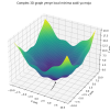
Na kumbuka neural networks inaweza kuwa na so many weights, hivyo hata graph / curve ya hii function ita produce very complex higher dimensional shapes

Mfano, kwa neural network rahisi yenye just two weights, hii itakua shape of its Error function (Error ikiwa function ya hizo weights)

Ni slightly complex graph for just two weights, kwa weights zaidi ya moja tunahamia kwenye higher dimensional shapes ambazo hatuwezi hata kuzi visualize
Kitu kingine cha msingi kuki note kwenye hio graph, ni kwamba japokua ni function ni complex ila ni differentiable

Najua bado hujasahau calculus, ila tukumbushane tuna maana gani tunaposema function ni differentiable

Function ni differentiable kama ina change smoothly as its variables change, hakuna mabadiliko ya ghafla (abrupt change) au jump at any point on the graph, so unaweza kuchora tangent line katika point yoyote ile unayotaka
Hivyo tunaweza kupima kwa kiasi gani kidogo sana function ina changes kama one of its varaible iki change, kwa maneno mengine tunaweza measure its rate of change, hence differentiable

Sasa twende kwenye point ya msingi, jinsi gani Gradient Descent ita solve hili tatizo? Na Gradient descent ni nini haswa?

Hii ni formal definition ya Gradient Descent

It is a first-order iterative algorithm for finding a local minimum of a differentiable multivariate function.

(Kama mara ya mwisho kusoma pure mathematics ni Advance, nadhani hii method hujawahi kukutana nayo, hivyo tuchukue mda kidogo kuielewa)

Tayari tunajua nini maana ya differentiable function (if we can calculate its rate of change, then it is differentiable), lakini tuna neno optimization, firs-order, iterative, a local minimum na multivariate function, ni vitu gani?

Ok, optimization ni method ya kutafuta "best" au most efficient solution kutoka kwenye set of many possible solutions or choices
Kuiweka kwenye mfano, imagine unataka ku budget mafuta kwenye gari lako wakati unasafiri kwenda sehemu A, kama kuna njia 7 za kupita ili ufike, optimization ni pale unapochagua njia fupi zaidi ya kupita kwasababu ndio itaokoa mafuta zaidi kuliko nyingine.

Nini maana ya local minimum? Ok, turudi back in time, Advance.

In differentiation, minimum point au points (jina lingine local minimum) ni thamani za variable(s) ambazo zina produce lowest possible value of the function

Imagine hii function

Minimum points ni value za x ambazo zinafanya y iwe ndogo, for single variable function kama hii tunaweza kupata minimum points kwa kufanya first order au first derivative (gradient) yake iwe 0
(Tunaposema first-order tuna maana ya first derivative of function au gradient)

So, kwenye 0,0 ndipo function, y inapokua na lowest value, hii ni graph ya y function ikionyesha hio minimum points au local minimum

Sawa, lakini utakutana na hii term nyingine ya Global minimum? kama maneno yanavyo suggest, local minimum ni point on the graph ambapo function inakua na lowest value BUT ukiilinganisha na nearby points, hence neno local

Kwa upande mwingine, Global minimum ni point on the graph ambapo function inakua na lowest value ukiilinganisha na all other points

Tukiiweka kwenye mfano wetu wa gari, local minimum ni ile njia fupi ukilinganisha na njia nyingine za karibu yake, ila global minimum ni ile njia fupi zaidi kuliko nyingine, ambayo ndio ya muhimu zaidi kwenye optimization ya mafuta

Function yetu ya

ni simple kiasi kwamba its local minimum ni sawa na its global minimum, hakuna point yoyote ile yenye lowest value of y ukiacha 0,0

Now, fikiria complex function ya complex graph kama hii

Kama una imagine hio curve kama bonde kubwa, then kuna vibonde vidogo vidogo (local minimum) vipo kwa ndani
Ila chini kabisa ya hili bonde ndio global minimum ya bonde lote, sehemu ambayo mwinuko (gradient) ni mdogo zaidi kuliko sehemu nyingine yoyote

Kwa very complex curve, ni ngumu kupata Global minimum (kufika chini kabisa ya bonde nikiiweka katika mfano), hivyo matumaini yetu ni angalau tutafute local minimum ambayo ipo karibu na global minimum

Nini maana ya iterative, gradient descent ni iterative kwasababu haitupatii local minimum (au global minimum kama tuna bahati) moja kwa moja, in one step, bali inarudia rudia in many steps mpaka inapojiamini kuwa imefika kwenye local minimum ya function

Sina haja ya kuelezea zaidi kuhusu Algorithm cause nahakika unajua maana yake, ila kwa meneno machache ni step-by-step solution to a problem

Multivariate function ni function yoyote ile inayo depend on many variables (au dimensions kwa jina lingine)
Mfano

ni multivariate function ya

na

. Hivyo gradient descent inaweza ku operate kwenye higher dimensional space

Nguvu ya Gradient descent ni kwamba, hatuna haja ya kujua function yenyewe ili kupata its local minimum kama ilivyokua kwa

Criteria ambayo kimsingi ina fit kwenye tatizo letu kwasababu hatujua actual equation ya Loss function yetu.
Kwa kutumia Gradient descent tunaweza estimates its local minimum bila haja ya ku derive na kuijua Loss function nzima (kwasababu hatuwezi hata hivyo)

Unaweza kujiuliza swali, hayo maelezo yote yanahusiana vipi na ku reduce Error au Loss function kitu ambacho ndio tunakitaka

Well, imagine kama our Loss function ni hii quadratic equation

Kutafuta local minimum yake ni sawa sawa kabisa na ku reduce its value, kwasababu hiyo ndiyo sifa ya local minimum, point ambayo function has the lowest value

Na ku reduce loss function ndio maana ya ku learn kwenye network, kwasababu kunakua hakuna tofauti kubwa kati ya output ya neural network na target value, tunasema neural network has learned

So kama tukiweza ku tafuta local minimum ya hii Complex and unknown Loss function kwa kutumia gradient descent tunaweza sasa ku train our neural network
Na kwasababu variables za hii loss function ni weights of network, gradient descent automatically ita calculate na ku assign correct value ya weights ambazo zitakua na uwezo wa ku produce correct value mwisho wa training

Kwa maneno mengine, gradient descent itaenda kututafutia values of weights ambazo zina reduce the Error au Loss function the most kitu ambacho tulikua tu struggle kukipata

Nasema the "most" not completely, kwasababu tuna deal na complex "valleys" au shapes in higher dimensional space, hivyo ni ngumu kupata global minimum, lakini gradient descent ni efficient enough kutupa local minimum ambayo ipo so close tu global minimum

Hivyo neural network haiwezi kuwa completely correct mara zote, lakini to be fair, hata binadamu tupo hivyo.

So how actually gradient descent work?

Gradient descent ina njia rahisi zaidi na intuitive ya ku solve tatizo letu la ku train neural network

Kuielewa, imagine hii scenario

Upo kwenye kilele cha bonde au mlima wenye vilele vingi (mfano wa complex Loss function yetu), lengo lako ni kushuka chini (to the local au global minima, ambapo error ina lowest value), lakini kuna tatizo.
Ni usiku na giza, huna ramani na hujui njia (Loss function is unkown)

Kitu pekee ulichonacho ni tochi inayoweza kumurika hatua tatu au nne mbele
Kwenye hii situation, Gradient descent algorithm inakwambia utazame sehemu ulipo kisha uangalie ni sehemu ipi kuna mwinuko, kisha uende opposite na hio sehemu

Kwa maneno mengine, tafuta sehemu ambayo inateremsha chini (descent), kinyume na mwinuko (opposite of the gradient), hii algorithm ni very intuitive, kimsingi inakwambia haijalishi ni sehemu ipi utajikuta kwenye hili bonde kwa kila hatua utakayopiga, usipandishe juu

Kwa kila sehemu utakayofika, rudia tena hii njia, murika tochi yako kutazama wapi kuna mwinuko, kisha wewe shuka chini
Ndiyo maana inaitwa Gradient descent (means, always take the steps opposite to the gradient or slope)
Kama ukifanya hii tena na tena (iteratively), utajikuta umefika chini ya bonde

Inaendelea hapa

 

[Kuchwizzy]

Inaendelea....

Kama Error function ingekua ni simple kama hii quadratic equation

Hivi ndivyo tunge arrive kwenye its local minimum (or local minima) kwa kutumia gradient descent

Kama tunavyoona, tunaenda in opposite direction of the gradient. na hii ndio point ya msingi kuikumbuka

Kama gradient ni negative (inashuka), we move to the right (we increase x), kama ni positive (inapanda) we move to the left (we decrease x)

Na wapi tunaanzia? Haijalishi tunaweza anza na random position, popote pale kwenye curve, gradient descent inatufikisha kwenye local minima haijalishi wapi tumeanzia

Kitu kingine ambacho gradient descent inatwambia ni kwamba, tunapokaribia kwenye local minimum tunapaswa ku takes small steps ili tusipapite (overshoot), tunapokua mbali na local minimum, tu take large steps kupawahi

Lengo ni ku avoid ku bounce over, na kucheza cheza around local minimum

Kama tulivyokwisha ona, very complex higher dimensional curve zinaweza kuwa na local minimum zaidi ya moja, so tutajua vipi kama tumefika kwenye correct local minimum?

Tuna solve hili tatizo, kwa ku train neural network yetu from different starting points au parameters, means at every iteration we will start with different values of weights

Tuchukue huu mda ku formalize vyote tulivyojifunza mpaka sasa

1. Gradient Descent:

• An iterative optimization algorithm used to find the local minimum of a multivariate differentiable. It works by repeatedly taking steps in the direction of the steepest descent (negative gradient) of the function at the current point.

2. First Order (in calculus):

• Refers to mathematical operations involving the first derivative of a function. First-order methods, like gradient descent, use information about the slope (gradient) of a function to guide their search for optimal points.

3. Iterative:

• A process that is repeated multiple times, with each repetition (iteration) building upon the results of the previous one. Gradient descent is iterative, as it updates its estimate of the minimum with each step.

4. Optimization:

• The process of finding the best solution from a set of possible solutions. In machine learning, this often involves finding the model parameters that minimize a loss function.

5. Multivariate:

• Involving multiple variables. In the context of machine learning, many models deal with datasets having multiple features or predictors, making them multivariate.

6. Algorithm:

• A step-by-step procedure or set of rules for solving a problem or accomplishing a task. Gradient descent is an example of an algorithm used for optimization.

7. Higher Dimensional Space (in context of machine learning):

• Refers to a space with more than three dimensions. In machine learning, models often work with data represented in high-dimensional spaces, where each feature corresponds to a dimension.

8. Local Minimum:

• A point where a function's value is lower than all nearby points, but not necessarily the lowest value across the entire function's domain.

9. Global Minimum:

• The point where a function attains its absolute lowest value across its entire domain.

10. Derivative:

• A measure of how a function changes as its input changes. The derivative at a point gives the slope of the tangent line to the function's graph at that point.
  
  
  
• "It is a first-order iterative algorithm for finding a local minimum of a differentiable multivariate function."
  1. First-Order:
     • Refers to the fact that the algorithm uses the first derivative (gradient) of the function to find the local minimum. It does not require the second derivative (Hessian matrix) for its calculations.
  2. Iterative:
     • Indicates that the algorithm improves its solution step-by-step, updating its estimate of the minimum in each iteration. It repeats the process until it converges to a solution or meets certain criteria.
  3. Algorithm:
     • A step-by-step procedure or set of rules designed to perform a specific task. In this context, it’s a method for finding the minimum of a function.
  4. Finding a Local Minimum:
     • The goal of the algorithm is to identify a point where the function value is lower than that of the points in its immediate vicinity. It aims to locate a "local" minimum, which is a point that may not be the absolute lowest (global minimum) but is the lowest within a certain region.
  5. Differentiable:
     • The function must be differentiable, meaning it has a well-defined derivative (gradient) at all points in its domain. This ensures that the algorithm can use the gradient information to guide its search.
  6. Multivariate Function:
     • The function depends on multiple variables (or dimensions).

NEXT : Mean Squared Error ( Loss ) Function And Mathematics of Gradient Descent Algorithm